
Deep Learning.ai - Andrew Ng
Review
Course Link
Info
This is a comprehensive course in deep learning by Prof. Andrew Ang, Stanford University, in Coursera. The course covers the three main neural network architectures, namely, feedforward neural networks, convolutional neural networks, and recursive neural networks. Their related applications, extensions, and tweaks are covered with sufficient example codes in Python, TensorFlow, and Keras. The specialisation uses Jupyter for its assignments.
Syllabus
This is a 5 course specialisation.
- Neural Networks and Deep Learning
- neural network in Numpy
- logistic regression, backpropagation
- Improving Deep Neural Networks: Hyperparameter Tuning, Regularization, and Optimization
- L2 and dropout regularization, weight initialization, batch normalization, gradient checking
- mini-batch gradient descent, Momentum, RMSprop and Adam
- neural network in TensorFlow
- Structuring Machine Learning Projects
- Convolutional Neural Networks
- convolutional neural networks in numpy and Keras
- Alex Net, VGG Net, Inception Net, Residual Net
- object detection, localization
- neural style transfer
- face recognition
- Sequence Models
- RNN, GRU, LSTM
Repository
The repository consists of the following:
- Projects - Jupyter notebook and Python codes
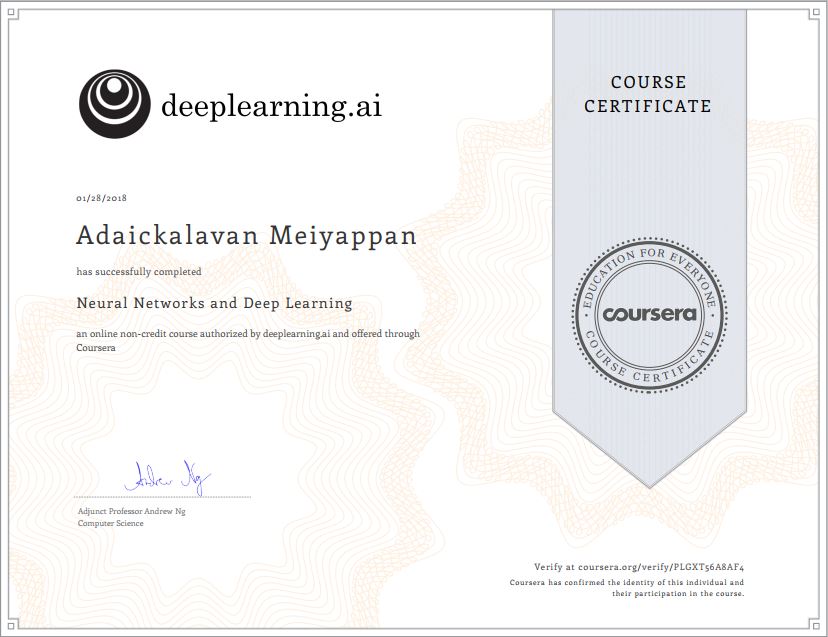
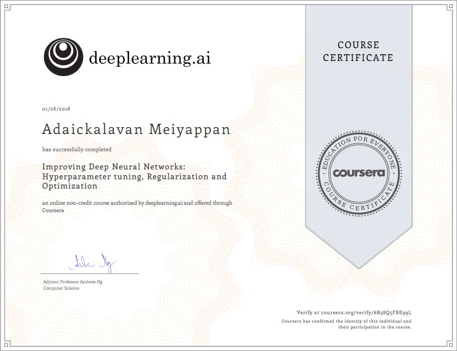
Verified Certificate
-
Neural Networks and Deep Learning
-
Improving Deep Neural Networks: Hyperparameter Tuning, Regularization, and Optimization
-
Structuring Machine Learning Projects
-
Convolutional Neural Networks
Notes
Some helpful hints are listed below.
- To download all the files for an assignment from Jupyter, do the following:
- In the Jupyter notebook, use the “+” button to insert a new cell.
- In the cell, add this code
# Linux !tar -cvzf all_files.tar.gz * # Windows !zip all_files.zip * - Hit Shift+Enter to run the cell
- Go to File -> Open -> ‘all_files.tar.gz’ -> Download
- The ‘all_files.tar.gz’ contains all the assignment files
Course 4: Convolutional neural networks
Week 2 Project: ResNets
A ResNet is implemented in this week’s assignment using Keras.
It may be helpful to gain a deeper understanding on the axis over which batch normalization is performed.
In feedforward NN, the tensor is of shape [m,z] where m is batch size, and z is number of features (i.e., output of linear unit). In batch normalization, we normalize over batch_size for each feature. So that gamma and beta have the same lengths/shape as the number of features z.
In CNN, the tensor is of shape [m,h,w,c] where m is batch size, h is height of image, w is width of image, c is number of channels. In batch normlaization, we normalize over batch_size*height*width for each channel. So that gamma and beta have the same lengths/shape as the channel. The following line of code in Keras X = BatchNormalization(axis = 3)(X) will compute mean of tensor X over axis 0, 1, and 2.
Below is a sample python code to illustrate the essence and differences in batch normalization process between a feedforward network and a convolutional network.
def batch_norm(X, gamma, beta, eps = 1e-5):

    """
    Arguments:
    X (for feedforward NN) -- input tensor of shape (m, z)
                           -- m is batch size
                           -- z is number of features
    X (for CNN) -- input tensor of shape (m, h, w, c)
                -- m is batch size
                -- h is height of image
                -- w is width of image
                -- c is number of channels
    gamma -- learnable variance parameter
    beta -- learnable mean parameter
    eps -- small number to prevent division by zero

    Returns:
    bn -- batch normalized data of same shape as input X
    """

    if len(X.shape) not in (2, 4):
        raise ValueError('only supports feedforward or convolutional neural network')

    # For feedforward neural network
    if len(X.shape) == 2:
        # mini-batch mean
        mean = nd.mean(X, axis=0)
        # mini-batch variance
        variance = nd.mean((X - mean) ** 2, axis=0)
        # normalize
        X_hat = (X - mean) * 1.0 / nd.sqrt(variance + eps)
        # scale and shift
        bn = gamma * X_hat + beta

    # For convolutional neural network
    elif len(X.shape) == 4:
        # extract the dimensions
        m, h, w, c = X.shape
        # mini-batch mean
        mean = nd.mean(X, axis=(0, 1, 2))
        # mini-batch variance
        variance = nd.mean((X - mean.reshape((1, 1, 1, c))) ** 2, axis=(0, 1, 2))
        # normalize
        X_hat = (X - mean.reshape((1, 1, 1, c))) * 1.0 / nd.sqrt(variance.reshape((1, 1, 1, c)) + eps)
        # scale and shift
        bn = gamma.reshape((1, 1, 1, c)) * X_hat + beta.reshape((1, 1, 1, c))

    return bn
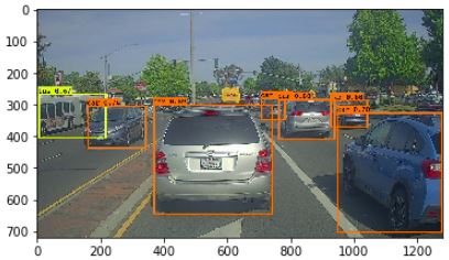
Week 3 Project: YOLO - Car detection
In exercise section 2.3 yolo_non_max_suppression, the provided python code performs non-max suppression (NMS) operation without taking into consideration the class labels of each box. Following is an example to illustrate the shortcoming of the given code in the exercise.
Assume there are 2 boxes with the following:
- Box1 is a car on one of the 19x19 cell with 0.99 probability
- Box2 is a person on the same cell (on a diff anchor box obviously) with 0.9 probability
- Box1 and Box2 has overlap > 0.5,
- Box2 will get suppressed. But ideally both boxes should had been retained since they are labelling different classes.
Ideally, the NMS operation should be performed once for every class. If a car and a pedestrian have their prediction boxes largely overlapped (and no other cars/pedestrians overlap them), then neither of them should get suppressed.
The function tf.image.non_max_suppression() does not have a class input to perform automatic class based NMS. Hence, we should gather boxes belonging to the same class and run tf.image.non_max_suppression() on each of the set indepently. In this manner we would be able to consider classes when doing NMS.
I have a provided a sample python code below to perform class based NMS. Please do share if you have a better vectorized implementation of class based NMS operation.
import numpy as np
import tensorflow as tf
from keras import backend as K

def yolo_non_max_suppression(scores, boxes, classes, max_boxes = 10, iou_threshold = 0.5):
    """
    Applies Non-max suppression (NMS) to set of boxes

    Arguments:
    scores -- tensor of shape (None,), output of yolo_filter_boxes()
    boxes -- tensor of shape (None, 4), output of yolo_filter_boxes() that have been scaled to the image size (see later)
    classes -- tensor of shape (None,), output of yolo_filter_boxes()
    max_boxes -- integer, maximum number of predicted boxes you'd like
    iou_threshold -- real value, "intersection over union" threshold used for NMS filtering

    Returns:
    selectedScores -- tensor of shape (, None), predicted score for each box
    selectedBoxes -- tensor of shape (4, None), predicted box coordinates
    selectedClasses -- tensor of shape (, None), predicted class for each box

    Note: The "None" dimension of the output tensors has obviously to be less than max_boxes. Note also that this
    function will transpose the shapes of scores, boxes, classes. This is made for convenience.
    """

    max_boxes_tensor = K.variable(max_boxes, dtype='int32') # tensor to be used in tf.image.non_max_suppression()
    K.get_session().run(tf.variables_initializer([max_boxes_tensor])) # initialize variable max_boxes_tensor

    #Round the prediction variable 'classes' to the nearest integer to make a firm class decision
    roundedClasses = tf.round(classes)
    #Uncomment the following line to verify correctness of code implementation
    #print('roundedClasses : {}'.format(roundedClasses.eval()))
    #Create the necessary lists
    numOfClass = 80 #number of classes available
    classNum = tf.constant(list(range(numOfClass)), shape=(numOfClass,1), dtype=tf.float32)
    selectedScores = []
    selectedBoxes = []
    selectedClasses = []
    for ii in range(numOfClass):
        #Retrieve indices of a given class from firm prediction variable 'roundedClasses'
        indices = tf.where(tf.equal(roundedClasses,classNum[ii]))[:,0]
        #Use K.gather() to select rows from scores, boxes and classes corresponding to the chosen class
        gatheredScores = K.gather(scores,indices)
        gatheredBoxes = K.gather(boxes,indices)
        gatheredClasses = K.gather(roundedClasses,indices)
        # Use tf.image.non_max_suppression() to get the list of indices corresponding to boxes you keep for a given class
        nms_indices = tf.image.non_max_suppression(gatheredBoxes, gatheredScores, max_boxes, iou_threshold)
        #Use K.gather() to select rows from scores, boxes and classes corresponding to the chosen class
        gatheredScores = K.gather(gatheredScores,nms_indices)
        gatheredBoxes = K.gather(gatheredBoxes,nms_indices)
        gatheredClasses = K.gather(gatheredClasses,nms_indices)
        #Combine NMS selected scores and boxes per class into a list
        selectedScores.append(gatheredScores)
        selectedBoxes.append(gatheredBoxes)
        selectedClasses.append(gatheredClasses)
        #Uncomment the following lines to verify correctness of code implementation
        #print('Indices of class {} : {}'.format(ii,indices.eval()))
        #print('Values of class {}: {}'.format(ii,gatheredClasses.eval()))

    #Concatenate the NMS selected scores, boxes, classes into tensor objects
    selectedScores=tf.concat(selectedScores,axis=0)
    selectedBoxes=tf.concat(selectedBoxes,axis=0)
    selectedClasses=tf.concat(selectedClasses,axis=0)
    #Uncomment the following lines to verify correctness of code implementation
    #print(selectedScores.eval())
    #print(selectedBoxes.eval())
    #print(selectedClasses.eval())

    return selectedScores, selectedBoxes, selectedClasses

tf.reset_default_graph()
np.random.seed(1)
mu = 1 #mean
sigma = 4 #standard deviation
tempScores = np.random.normal(mu, sigma, [54,])
tempBoxes = np.random.normal(mu, sigma, [54, 4])
tempClasses = np.random.uniform(0, 80, [54,])
scores = tf.cast(tempScores,tf.float32)
boxes = tf.cast(tempBoxes,tf.float32)
classes = tf.cast(tempClasses,tf.float32)

with tf.Session() as test_b:
    scores, boxes, classes = yolo_non_max_suppression(scores, boxes, classes)
Course 5: Sequence models
Week 1 Project: Bulding RNN - step by step
In Section 3.2, the original equations 7 to 17, are erroneous. The correct equations are given below:
3.2.2 gate derivatives
\(d\Gamma_f^{\langle t \rangle} = dc_{next}*\tilde c_{prev} + \Gamma_o^{\langle t \rangle} (1-\tanh(c_{next})^2) * c_{prev} * da_{next}\tag{7}\) \(d\Gamma_u^{\langle t \rangle} = dc_{next}*\tilde c^{\langle t \rangle} + \Gamma_o^{\langle t \rangle} (1-\tanh(c_{next})^2) * \tilde c^{\langle t \rangle} * da_{next}\tag{8}\) \(d\tilde c^{\langle t \rangle} = dc_{next}*\Gamma_u^{\langle t \rangle}+ \Gamma_o^{\langle t \rangle} (1-\tanh(c_{next})^2) * \Gamma_u^{\langle t \rangle} * da_{next} \tag{9}\) \(d \Gamma_o^{\langle t \rangle} = da_{next}*\tanh(c_{next})\tag{10}\)
3.2.3 parameter derivatives
\(dW_f = d\Gamma_f^{\langle t \rangle} * \Gamma_f^{\langle t \rangle}*(1-\Gamma_f^{\langle t \rangle}) * \begin{pmatrix} a_{prev} \\ x_t\end{pmatrix}^T \tag{11}\) \(dW_u = d\Gamma_u^{\langle t \rangle} * \Gamma_u^{\langle t \rangle}*(1-\Gamma_u^{\langle t \rangle}) * \begin{pmatrix} a_{prev} \\ x_t\end{pmatrix}^T \tag{12}\) \(dW_c = d\tilde c^{\langle t \rangle} * (1-(\tilde c)^2) * \begin{pmatrix} a_{prev} \\ x_t\end{pmatrix}^T \tag{13}\) \(dW_o = d\Gamma_o^{\langle t \rangle} * \Gamma_o^{\langle t \rangle} * (1-\Gamma_o^{\langle t \rangle}) * \begin{pmatrix} a_{prev} \\ x_t\end{pmatrix}^T \tag{14}\)
To calculate $db_f, db_u, db_c, db_o$ you just need to sum across the horizontal (axis= 1) axis on $d\Gamma_f^{\langle t \rangle}, d\Gamma_u^{\langle t \rangle}, d\tilde c^{\langle t \rangle}, d\Gamma_o^{\langle t \rangle}$ respectively. Note that you should have the
keep_dims = Trueoption.Finally, you will compute the derivative with respect to the previous hidden state, previous memory state, and input. \(da_{prev} = W_f^T*d\Gamma_f^{\langle t \rangle} + W_u^T * d\Gamma_u^{\langle t \rangle}+ W_c^T * d\tilde c^{\langle t \rangle} + W_o^T * d\Gamma_o^{\langle t \rangle} \tag{15}\) Here, the weights for equations 15 are the first n_a, (i.e. $W_f = W_f[:, : n_a]$ etc…) \(dc_{prev} = dc_{next}\Gamma_f^{\langle t \rangle} + \Gamma_o^{\langle t \rangle} * (1- \tanh(c_{next})^2)*\Gamma_f^{\langle t \rangle}*da_{next} \tag{16}\) \(dx^{\langle t \rangle} = W_f^T*d\Gamma_f^{\langle t \rangle} + W_u^T * d\Gamma_u^{\langle t \rangle}+ W_c^T * d\tilde c_t + W_o^T * d\Gamma_o^{\langle t \rangle}\tag{17}\) where the weights for equation 17 are from n_a to the end, (i.e. $W_f = W_f[:, n_a :]$ etc…)
In Section 3.3, the expected result for lstm_backward function seem to be incorrect. A few key points to note in completing the lstm_backward function:
da[:,:,t]is the gradient of the loss at present time $\langle t \rangle$ with respect to hidden state at present time $\langle t \rangle$da_prevtis the accumulated gradient of the loss from time time $\langle T_x \rangle$ to $\langle t-1 \rangle$ with respect to hidden state at present time $\langle t \rangle$- Add the
da_prevttoda[:,:,t]when feeding into thelstm_cell_backwardfunction:gradients = lstm_cell_backward(da[:,:,t] + da_prevt, dc_prevt, caches[t]) - Remember to update the values of
da_prevtanddc_prevtat each time:dc_prevt = gradients["dc_prev"] da_prevt = gradients["da_prev"]
Leave a comment