
Artificial Intelligence - Ansaf Salleb-Aouissi
Review
Course Link
Artifical Intelligence - Ansaf Salleb-Aouissi
Info
This course on artificial intelligence mirrors much of the syllabus from the book Artificial Intelligence: A Modern Approach” - Stuart Russel and Peter Norvig. The course is well articulated by Prof. Ansaf Salleb-Aouissi, University of Columbia, in EdX. The class has 5 programming assignments which translates the theory learnt to solving real-life problems.
Syllabus
Uninformed/heuristic/adversarial search, constraint satisfaction, perceptron, k-NN, neural networks, support vector machine, decision trees, Markov decision processes, reinforcement learning, logical/propositional agent, applications to natural language processing and vision
Verified Certificate

Week 2 Project: Search Algorithms
We are to implement a breadth-first search (BFS), depth-first search (DFS), and A* search to solve an 8-puzzle game. The pseudo codes for all 3 algorithms are given in the course lecture notes. To complete the assignment, a simple implementation of the given pseudocode is sufficient.
In order to meet the execution time constraints, there are several key points to note as follows.
-
Use
class treeto represent a tree which depends on nodes created fromclass node. This keeps the code clean and efficient. -
Use
stringto store the state of each node, instead of lists or arrays. For example, storestateStr = "21345670"as a string to denote a node state. String comparison is faster than list/array comparison. -
Store the explored states’ strings in a set :
exploredStates = set(). PerformexploredStates.isdisjoint({childStateStr})to check whether the current child state stringchildStateStrexists within the explored states’ strings. -
Use string based states for comparison and a list based states to reorder state elements when moving to another state. For example, use lists to change
[2, 1, 3, 4, 5, 6, 7, 0] --> [1, 2, 3, 4, 5, 6, 7, 0]. It is easier to manipuate state elements in a list form. It may be useful to know how to iterate between a string and a list in your code.
  #Convert list to string: StateList ---> StateStr
  stateStr = ''.join(stateList)
  print(stateStr)

  #Convert string to list: StateStr ---> StateList
  stateList = list(stateStr)
  print(stateList)
- A memory and time efficient implementation of priority queue is needed for A* algorithm. I have implementaed my own below which uses a dual representation of the priority queue in the form of a list and a dictionary. It has two functions, namely, push and pop to place and get items from the queue, respectively. The priority queue:
- Orders and re-orders items according to their priority
- Removes duplicate entries with lower priority upon the addition of higher priority entries
- Uses the first entry if there are duplicate entries with the same priority value
- My priority queue implementation, with comments:
 class priorityQueue():
     def __init__(self):
         self.qList = [] #frontier state in a heap list
         self.qDict = {} #frontier state strings
         self.index = 0 #unique sequence count

     def pushObject(self, priority, item):
         #Add new object or update priority of existing object in qDict dictionary
         self.index += 1
         if item.stateStr in self.qDict: #If the item exist in frontier
             itemOld = self.qDict[item.stateStr]
             if item.cost < itemOld.cost:
                 self.qDict[item.stateStr] = item
                 # Simply add the new node (with a higher priority) without
                 # removing the existing node (with lower priority).
                 heapq.heappush(self.qList,[priority,self.index,item])
         else: #If the item does not exist in frontier
             self.qDict[item.stateStr] = item
             # Simply add the new node (with a higher priority) without
             # removing the existing node (with lower priority).
             heapq.heappush(self.qList,[priority,self.index,item])

     def popObject(self):
         #Remove and return item wth the highest priority task.
         while True:
             cost0, index0, item0 = heapq.heappop(self.qList)
             if item0.stateStr in self.qDict:
                 del self.qDict[item0.stateStr]
                 break
             else:
                 #Remove duplicate nodes in self.qList with lower priority
                 #(introduced by addObject function) which already have been
                 #explored previously.
                 pass

         return item0
Week 4 Project: Adversarial Search and Games
We are to solve the 2048 problem using the minimax algorithm with alpha-beta pruning. The algorithm is given in course lecture notes. You may try playing the 2048 game here and practice the alpha-beta pruning algorithm here.
Although this programming assignment is claimed to be the toughest in this course, it appears the be pretty starightforward.
- Implement the pseudocode from the course lecture notes
- Design a heuristic to evaluate the utility
Some good heuristics for solving 2048 are discussed at this thread. Key to devising a good heuristic is to ensure the heuristics do not have significant overlap or have low degrees of correlation. Keeping the heuristic simple is really helpful to this end. In my project, I used only two heuristics, namely, number of remaining free tiles and smoothness.
- Higher number of remaining free tiles imply
- increased count of tile merges, thus higher valued tiles
- longer gameplay, thus leading to higher valued tiles
- Smoothness is the sum of absolute value difference between adjacent tiles. Minimizing the difference results in tiles being arranged in a monotonic order (sprouting from a corner) making tile merges more likely. In fact, smoothness is the king in heuristics for the 2048 game. For experimental results proving this claim, refer here
It is important to normalize the 2 heuristics first. The number of remiaing free tiles was divided with the total number of tiles (i.e., 4x4 = 16) and the total smoothness value was divided by the total sum of all tiles on grid. Hence, we have our final heuristic \(h\) function to be
\[\begin{align*} h_1 & = \frac{number\_of\_free\_tiles}{total\_number\_of\_tiles} \\ h_2 & = \frac{sum\_of\_all\_differences}{sum\_of\_all\_tile\_values} \\ h & = h_1 - h_2 \\ \end{align*}\]A max depth search of 4 levels and a time limit of 0.18 seconds is used, since a time limit for each move is imposed by the assignment instructions.
Below is my execution result for my heuristics, achieving full marks of 100%.
[Executed at: Sun May 28 4:14:32 PDT 2017]

Results of 10 trials:

Trials with max tile of 2: 0 %
Trials with max tile of 4: 0 %
Trials with max tile of 8: 0 %
Trials with max tile of 16: 0 %
Trials with max tile of 32: 0 %
Trials with max tile of 64: 0 %
Trials with max tile of 128: 0 %
Trials with max tile of 256: 0 %
Trials with max tile of 512: 10 %
Trials with max tile of 1024: 10 %
Trials with max tile of 2048: 60 %
Trials with max tile of 4096: 20 %
Trials with max tile of 8192: 0 %
Trials with max tile of 16384: 0 %
Trials with max tile of 32768: 0 %
Trials with max tile of 65536: 0 %
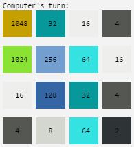
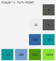
Pictures of my completed 2048 board
Code describing my heuristics implementation is as follows, which is only 11 lines long!
def evaluateUtility(grid):
    #Number of empty cells. Higher -> better
    totCell = len(grid.getAvailableCells())
    h1 = totCell/(grid.size*grid.size)

    #Smoothness of tiles. Lower -> better
    totDiff = 0
    #Along each column
    for i in range(grid.size - 1):
        totDiff += sum(list(map(absSub, grid.map[i], grid.map[i+1])))
    #Along each row
    for i in range(grid.size):
        totDiff += sum(list(map(absSub, grid.map[i][:-1], grid.map[i][1:])))

    totCell = sum(itertools.chain.from_iterable(grid.map))
    h2 = totDiff/(2*totCell) #Divided by 2 to ensure maximum normalised value is 1

    return h1 - h2
Week 7 Project: Machine Learning
On some given test data, we are to implement
- perceptron,
- linear regression, and
- classification, via
- SVM (polynomial kernel, RBF kernel),
- logistic regression,
- kNN,
- decision trees
- random forest machine learning agorithms using SciKit-Learn library, which is included in the standard Python distribution.
Perceptron
Simply implement the perceptron algorithm given on Slide 9, Lecture 6a:
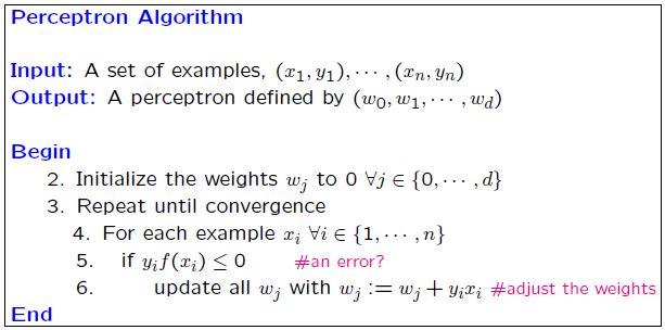
A sample decision bundary drawn by the perceptron learning lagorithm on the test data:
Linear regression
We are to normalize the input features (i.e., age, weight, height) and apply a gradient descent linear regression model for different step sizes and iteration counts. Simply implement a linear regression equation according to the given formulas in the project instruction notes.
As an additional problem, we are to choose an ideal learning rate and iteration count for the linear regression model. This basically amounts to choosing the minimum number of iterations taken to reach the minimum cost function value (i.e., empirical risk \(R(\beta)\)) made possible by a real valued step size. Simply iterate the linear regression model over various step sizes to find the optimum answer. Mine was \(\alpha=0.98\) and minimumIteration = 58.
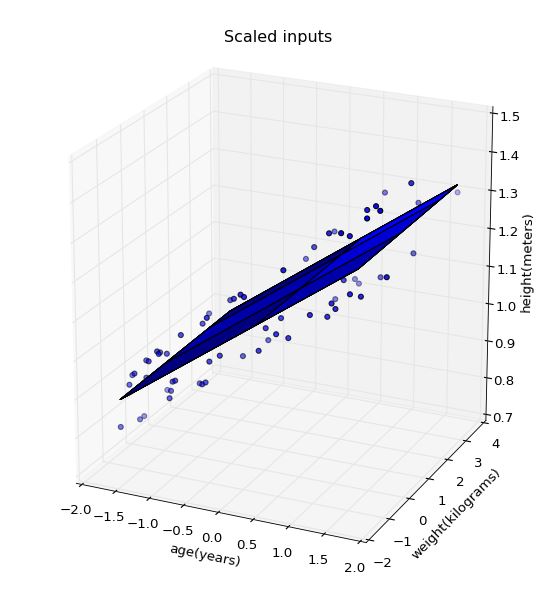
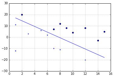
Next, we are to visualize the 2d planar decision boundary using matplotlib in a 3d space. Remember the regression coeeficients \(\widehat{\beta}\) which we calculated were obtained using normalized input features, \(z_j\) (or \(x_{scaled}\) in the project instruction notes). Hence, plotting the 2d plane will appear as shown on the left image below.
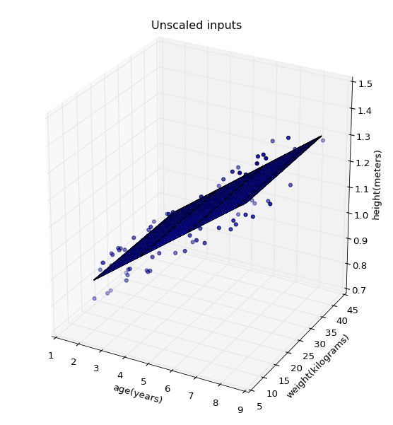
Obviously, the scales of the axes on the left image still uses normalized input feature values. To plot on axes using non-normalized feature values, such as that shown in the right image, we need to find the regression coefficients \(\beta\) for the non-normalized regression model.
We can transform the regression coefficients \(\widehat{\beta}\) from scaled inputs back to the non-normalized model via the following formula:
\[\begin{align} \beta_0 &= \widehat{\beta}_0-\sum_{j=1}^k\widehat{\beta}_j\frac{\overline{x}_j}{\sigma_j} \\ \beta_j &= \frac{\widehat{\beta}_j}{\sigma_j} \end{align}\]Derivation is given below.
We assume the following equation form for a regression model using normalized features (i.e., normalized regressors)
\[\begin{equation} y=\widehat{\beta}_0+\sum_{j=1}^k\widehat{\beta}_jz_j,\label{eq:7.1} \end{equation}\]where $\widehat{\beta}_j$ and \(z_j\) are the \(j\)-th regression coeeficient (i.e., weight) and \(j\)-th normalized feature, respectively. \(\widehat{\beta}_0\) is the bias and the filter length is \(k+1\). Here, \(z_j\) is generated from actual feature \(x_j\) by subtracting the sample mean \(\overline{x}_j\) and dividing by the sample standard deviation \(\sigma_j\):
\[\begin{equation} z_j = \frac{x_j-\overline{x}_j}{\sigma_j} \label{eq:7.2} \end{equation}\]Note that only the features had been normalized while the expected output/label \(y\) is not normalized. Now, substituting \eqref{eq:7.2} into \eqref{eq:7.1}, we have
\[\begin{equation} y=\widehat{\beta}_0+\sum_{j=1}^k\widehat{\beta}_j\left(\frac{x_j-\overline{x}_j}{\sigma_j}\right) \label{eq:7.3} \end{equation}\]Re-arranging, this expression can be written as
\[\begin{equation} y=\left(\widehat{\beta}_0-\sum_{j=1}^k\widehat{\beta}_j\frac{\overline{x}_j}{\sigma_j}\right)+\sum_{j=1}^k\widehat{\beta}_j\left(\frac{1}{\sigma_j}\right)x_j \label{eq:7.4} \end{equation}\]An equivalent equation form for a non-normalized regression model using actual feature values is
\[\begin{equation} y=\beta_0+\sum_{j=1}^k\beta_jx_j, \label{eq:7.5} \end{equation}\]where \(\beta_j\) is the \(j\)-th regression coeeficient (i.e., weight).
In order to obtain the unscaled regression coefficient, \(\beta\), from the scaled regression coefficent, \(\widehat{\beta}\), we compare \eqref{eq:7.5} with \eqref{eq:7.4}, to see that
\(\begin{align} \beta_0 &= \widehat{\beta}_0-\sum_{j=1}^k\widehat{\beta}_j\frac{\overline{x}_j}{\sigma_j} \\ \beta_j &= \frac{\widehat{\beta}_j}{\sigma_j} \end{align}\) \(\tag*{$\blacksquare$}\)
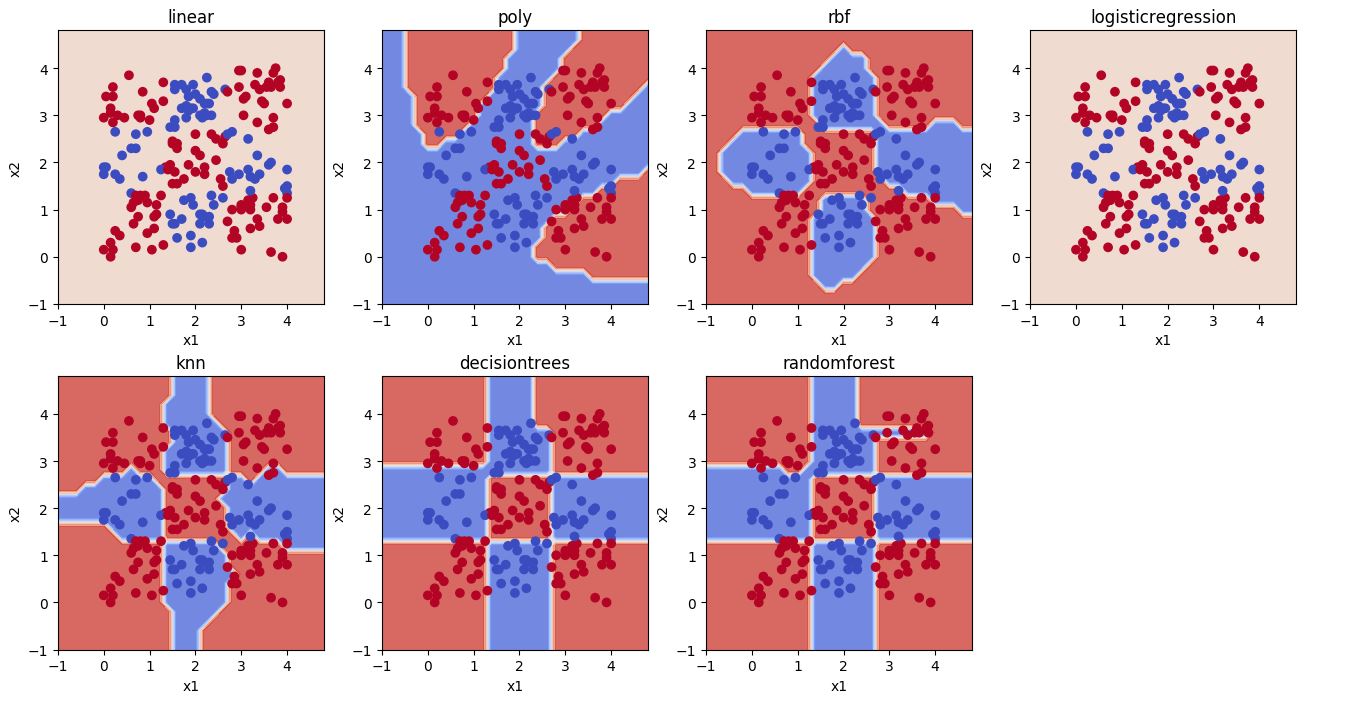
Classification
Here, we simply use the sklearn package to implement the various machine learning algorithms. A sample plot of the test data and the decision boundary produced by the various classifiers is shown below.
Week 9 Project: Constraint Satisfaction Problems
We are to solve a sudoku board by formulating the problem as a constraint satisfaction problem.
First, implement the AC-3 algorithm (arc consistency) according to the pseudocode given on Slide 59, Lecture 8.
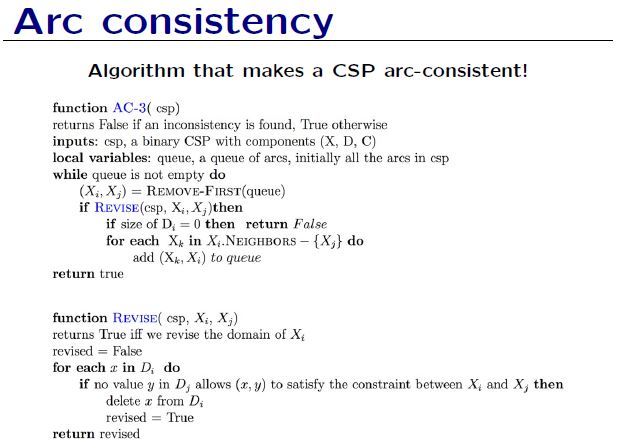
A constraint is represented as \(C_x\) != \(C_y\) (value in cell \(x\) not equal to value in cell \(y\)), where a cell is one of the 81 squares on the board. Every square on the board must have a different value than the squares in its row, its column, and its box (the local 3x3 grid). Therefore, each cell has 20 constraints with other cells (3x8 = 24, but 4 are duplicates, leaving 20 unique ones). Therefore, there are 81*20 = 1620 constraints in total.
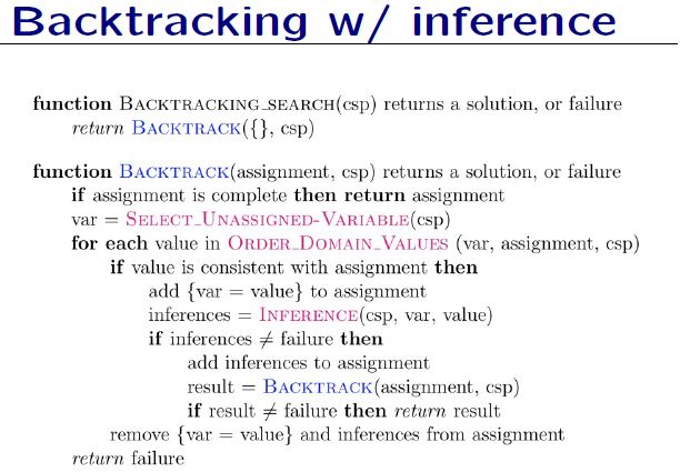
Next, implement the backtracking search algorithm with forward checking inference. Remember to use arc consistency check on the sudoku board initially as a preprocessing step before feeding the sudoku board into the BTS with inference algorithm. Using arc consistency check as a preprocessing step dramatically reduces the combination of values to be checked (i.e., reduces depth of BTS tree) and thus hastens the BTS algorithm. Pseudocode for BTS algorithm with inference is given on Slide 61, Lecture 8.
A few things to remember in optimizing the run-time of your code:
- Iterating through dictionary.items() would be faster than iterating through keys and accessing elements by them.
- A dict comprehension would be faster than adding each new value separately.
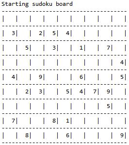
It is helpful to visualize the sudoku board. A handy function to visualize the sudoku board is provided below.
def visualizeBoard(sudokuAssign):
    #Prints a sudoku grid containing the assigned variables.
    #This function accepts a dictionary of the form:
    #sudokuAssign = {'A1':1, 'A2':4, 'A3':8, 'A4':0, 'A5':0, 'A6':7, 'A7':5, 'A8':0, 'A9':3,
    #                'B1':3, 'B2':0, 'B3':2, 'B4':0, 'B5':4, 'B6':0, 'B7':9, 'B8':0, 'B9':1,
    #                   :
    #                   :
    #                'I1':2, 'I2':8, 'I3':4, 'I4':0, 'I5':6, 'I6':0, 'I7':0, 'I8':3, 'I9':9,}
    #'0' values indicate unassigned variables and will not be printed.
    s = ""
    line = "-------------------------------------\n"
    s += line
    for row in "ABCDEFGHI":
        s += "|"
        for col in "123456789":
            if sudokuAssign[row + col] != 0:
                s += ("%3d" % sudokuAssign[row + col]) + "|"
            else:
                s += ("%3c" % ' ') + "|"
        s += "\n" + line

    print(s)
The above visualizeBoard function produces sudoku boards as shown below:
The testcases used by the vocareum grader were obtained in the report provided when I submitted my code for grading. The report, including the testcases, is reproduced below.
[Executed at: Thu Jul 13 10:58:36 PDT 2017]

003020600900305001001806400008102900700000008006708200002609500800203009005010300 [5/5]
500400070600090520003025400000000067000014800800600000005200000300007000790350000 [5/5]
000000000047056000908400061000070090409000100000009080000000007000284600302690005 [5/5]
000000000000530041600412005900000160040600002005200000000103200000005089070080006 [5/5]
090060000004000006003000942000200000086000200007081694700008000009510000050000073 [5/5]
000070360301000000042000008003006400004800002000003100005080007200760000000300856 [5/5]
000102900103097000009000070034060800000004500500021030000400000950000000000015307 [5/5]
800000090075209080040500100003080600000300070280005000000004000010027030060900020 [5/5]
000002008401006007002107903007000000065040009004000560000001000008000006910080070 [5/5]
006029000400006002090000600200005104000000080850010263000092040510000000000400800 [5/5]
000000000010720000700014826000000000006000900041906030050001000020097680000580009 [5/5]
005100026230009000000000000000900800590083000006500107060000001004000008853001600 [5/5]
680400000000710009013000000800000300000804090462009000000900037020007108000000026 [5/5]
000900007020007061300810002000078009007300020100040000000000050005000003010052078 [5/5]
000000060000130907900200031002000000004501703010006004046000020000010000200605008 [5/5]
000000000000002891080030507000000000047001085006427003000000000030005070719000204 [5/5]
010050000362010005070206400000005070005090600900000000700001008000374900601000000 [5/5]
000001086076300502000009300007000060900000800054000207008035900030900000000407000 [5/5]
307009000000003060006400001003100094025040803060300002000000006000200900580000040 [5/5]
021000050000000708000400020000600035060000000083020600059002086030001000006904200 [5/5]
Week 11 Project: Natural Language Processing
In this last programming assignment, we are tasked with developing a stochastic gradient descent based linear regression on transformed text data, for positive/negative sentiment classification of text. The text is transformed using unigram, bigram, and tf-idf text representation methods.
Key libraries to use for this assignment are
from sklearn.feature_extraction.text import CountVectorizer
from sklearn.feature_extraction.text import TfidfVectorizer
from sklearn.linear_model import SGDClassifier
During data prepocessing, besides removing common English stopwords, it is good to remove unnecessary punctuation marks and symbols.
def processText(text):
    global stopWordSet
    #Replace unwanted characters with spaces
    replacedText = text.replace('<br />', ' ')
    #Remove all punctuation marks
    chars = ".,?!;:-_/<>~`@#$%^&*()+=[]{}|\\\"\'"
    for c in chars:
        replacedText = replacedText.replace(c,' ')
    #Convert string into a list of words
    replacedTextList = replacedText.split()
    #Remove stopwords from the list of words
    processedText = ' '.join([word for word in replacedTextList if word.lower() not in stopWordSet])

    return processedText
For unigram and unigram-tfidf text representation, we use ngram = 1 in obtaining the text representation. But, in order to obtain good prediction accuracy for bigram and bigram-tfidf text representation, we use both ngram = 1 and ngram = 2 (i.e., one and two word sequences) in obtaining the text representation. For example, set
- ngram_val = 1 for unigram and unigram-tfidf
- ngram_val = 2 for bigram and bigram-tfidf
in the code below
if tfidf:
    vectorizer = TfidfVectorizer(ngram_range = (1,ngram), stop_words = stopWordList)
else:
    vectorizer = CountVectorizer(ngram_range = (1,ngram), stop_words = stopWordList)
Leave a comment