
Real Time Streaming Visualization
Project
Problem
In this project we will develop a web based visualization tool for real time data streaming application. For the purpose of explanation, we shall assume that we are streaming data from a sensor, on which we perform some computation and subsequently classify the sensor data at each time point.
Our example will demonstrate the following:
- Running a Bokeh server
- Simultaneously running multiple python threads for other tasks
- Auto start of threads by simply starting the Bokeh server
- Interactions among: browser \(\longleftrightarrow\) server \(\longleftrightarrow\) pyhton threads
The following will be used:
- Python 3.6
- Multithreaded Python coding
- Bokeh plots
- Bokeh server
- PyCharm
It is recommended to use PyCharm as the IDE since it provides version control capability and project file structure management capability.
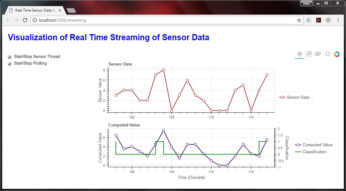
The expected end product of this project is shown below:
Repository
The repository consists of the following:
- Python and Bokeh scripts - complete functioning sample code
- .idea files - project setting files derived from PyCharm IDE
The project structure is as follows:
Real-Time-Streaming-Visualization   -- main folder
└── streaming                       -- python package, this is set as 'Source Root' in PyCharm
    ├── __init__.py                 -- this file indicates that 'streaming' is a python package
    ├── main.py                     -- script with main function
    ├── Sensor.py                   -- multithreaded python script to obtain sensor data
    └── Visual.py                   -- Bokeh code for web dashboard
Solution
It is beneficial for beginners to read through the Bokeh tutorial and guide to gain a better understanding of the visualization tool.
Begin with installation of Bokeh via the command: conda install bokeh (if you are using Anaconda python distribution, which is desirable) or pip install bokeh.
The code will be explained in a top to bottom manner. Hence, even if some parts are not clear at first, it will become clear towards the end when considering the various code as a whole system.
Firstly, we take a look at the main.py file.
from Visual import *
from Sensor import *

def threads(callbackFunc, running):
    # Set multiple threads
    sensor = Sensor(callbackFunc=callbackFunc, running=running) # Instantiate the Sensor thread
    # Start threads
    sensor.start() # Run the thread to start collecting data

def main():
    #Set global flag
    event = threading.Event() # Create an event to communicate between threads
    event.set() # Set the event to True

    webVisual = Visual(callbackFunc=threads, running=event) # Instantiate a Bokeh web document
    threads(callbackFunc=webVisual, running=event) # Call Sensor thread

# Run command:
# bokeh serve --show streaming
main()
Here, we do the following:
- Create a threading event to be used as Flag for communication between threads in python
- Instantiate a Bokeh web document as
webVisual, which is defined inVisual.pyfile - Instantiate our Sensor thread and run it
- For callback and interactive user experience:
- Feed the
threadsfunction intowebVisualobject to restart the thread from browser interface - Feed the Bokeh document
webVisualinto our thread to enable the Sensor thread to inform the browser whenever new sensor data is available for plotting - Feed the threading event Flag to both the Sensor thread and webVisual as a common Flag
- Feed the
To run this program, open a command prompt and change your present directory to that of the main folder, for example C:\Real-Time-Streaming-Visualization. Then issue the command bokeh serve --show streaming which will publish Bokeh document webVisual to a web browser at http://localhost:5006/streaming.
Secondly, we take a look at our Sensor thread which is defined in a threading.Thread class in Sensor file.
import time
import threading
import random
from functools import partial

class Sensor(threading.Thread):
    def __init__(self, callbackFunc, running):
        threading.Thread.__init__(self) # Initialize the threading superclass
        self.val = 0 # Set default sensor data to be zero
        self.running = running # Store the current state of the Flag
        self.callbackFunc = callbackFunc # Store the callback function

    def run(self):
        while self.running.is_set(): # Continue grabbing data from sensor while Flag is set
            time.sleep(0.2)  # Time to sleep in seconds, emulating some sensor process taking time
            self.val = random.randint(0, 10) # Generate random integers to emulate data from sensor
            self.callbackFunc.doc.add_next_tick_callback(partial(self.callbackFunc.update, self.val)) # Call Bokeh webVisual to inform that new data is available
        print("Sensor thread killed") # Print to indicate that the thread has ended
Here, the following is performed:
- When
sensor.start()is executed frommain.pyfile, therun()function in Sensor thread will be executed. - Sensor thread runs continuously as long as the Flag is set
- Random numbers are generated to emulate sensor data
- Once new sensor data is available, the webVisual object is called via Bokeh’s callback utility
add_next_tick_callback- In the callback, specifically invoke the
updatefunction of theVisualclass - Feed the necessary argument (i.e., new sensor data which is available in
self.val) to theupdatefunction by using a partial function
- In the callback, specifically invoke the
Refer to Bokeh guide on threads for more information on updating from threads. All actions from threads that update Bokeh document state must go through a add_next_tick_callback.
Finally, we see the python code to generate the Bokeh plots, Bokeh web document, and Bokeh Server which serves us the web based visualization.
from bokeh.plotting import figure
from bokeh.models import LinearAxis, Range1d, HoverTool, ColumnDataSource, Legend
from bokeh.layouts import gridplot, column, row
from bokeh.models.widgets import CheckboxGroup, Div
from bokeh.io import curdoc
from tornado import gen

class Visual:
    def __init__(self, callbackFunc, running):
        self.text1 = Div(text="""<h1 style="color:blue">Visualization of Real Time Data Streaming</h1>""", width=900, height=50) # Text to be displayed at the top of the webpage
        self.running = running # Store the current state of the Flag
        self.callbackFunc = callbackFunc # Store the callback function
        self.hover = HoverTool(  # To show tooltip when the mouse hovers over the plot data
                tooltips=[
                    ("index", "$index"), # Show index of plot data points
                    ("(x,y)", "(@x, $y)") # Show x and y coordinates of the plot data points
                ]
            )
        self.tools = "pan,box_zoom,wheel_zoom,reset" # Set pan, zoom, etc., options for the plot
        self.plot_options = dict(plot_width=800, plot_height=200, tools=[self.hover, self.tools]) # Set plot width, height, and other plot options
        self.updateValue = True # Internal state for updating of plots
        self.source, self.pAll = self.definePlot() # Define various plots. Return handles for data source (self.source) and combined plot (self.pAll)
        self.doc = curdoc() # Save curdoc() to make sure all threads see the same document. curdoc() refers to the Bokeh web document
        self.layout() # Set the checkboxes and overall layout of the webpage
        self.prev_y1 = 0

    def definePlot(self):
        # Define plot 1 to plot raw sensor data
        p1 = figure(**self.plot_options, title="Sensor Data")
        p1.yaxis.axis_label = "Sensor Value"
        # Define plot 2 to plot (1) processed sensor data and (2) classification result at each time point
        p2 = figure(**self.plot_options, x_range=p1.x_range, title="Computed Value") # Link x-axis of first and second graph
        p2.xaxis.axis_label = "Time (Discrete)"
        p2.yaxis.axis_label = "Computed Value"
        p2.extra_y_ranges = {"class": Range1d(start=-1, end=2)} # Add a secondary y-axis
        p2.add_layout(LinearAxis(y_range_name="class", axis_label="Classification"), 'right') # Name and place the secondary y-axis on the right vertical edge of the graph
        # Define source data for all plots
        source = ColumnDataSource(data=dict(x=[0], y1=[0], y2=[0], y3=[0]))
        # Define graphs for each plot
        r1 = p1.line(x='x', y='y1', source=source, color="firebrick", line_width=2) # Line plot for sensor raw data
        r1a = p1.circle(x='x', y='y1', source=source, color="firebrick", fill_color="white", size=8)  # Circles to indicate data points in first graph
        r2 = p2.line(x='x', y='y2', source=source, color="indigo", line_width=2) # Line plot for computed values
        r2a = p2.circle(x='x', y='y2', source=source, color="indigo", fill_color="white", size=8) # Circles to indicate data points in second graph
        r3 = p2.step(x='x', y='y3', source=source, color="green", line_width=2, y_range_name="class") # Overlay step plot for binary classes in the second graph
        # Place legends outside the plot area for each data source
        legend = Legend(items=[("Sensor Data", [r1, r1a])], location=(5, 30))
        p1.add_layout(legend, 'right')
        p1.legend.click_policy = "hide" # Plot line may be hidden by clicking the legend marker
        legend = Legend(items=[("Computed Value", [r2, r2a]), ("Classification", [r3])], location=(5, 30))
        p2.add_layout(legend, 'right')
        p2.legend.click_policy = "hide"  # Plot line may be hidden by clicking the legend marker
        # Combine all plots into a gridplot for better vertical alignment
        pAll = gridplot([[p1], [p2]])

        return source, pAll # Return handles to data source and gridplot

    @gen.coroutine
    def update(self, val):
        if self.updateValue: # Update the plots only if the 'self.updateValue' is True
            # Compute new values for each column data
            newx = self.source.data['x'][-1] + 1 # Increment the time step on the x-axis of the graphs
            newy1 = val # Assign raw sensor data to be displayed in the first graph
            newy2 = (val + self.prev_y1)/2 # Perform computation (i.e., moving average) on the sensor data and plot in the second graph
            self.prev_y1 = newy1
            newy3 = newy2 > 5 # Classify the signal (i.e., binary calssification) at each time point and plot the results in the second graph
            # Construct the new values for all columns, and pass to stream
            new_data = dict(x=[newx], y1=[newy1], y2=[newy2], y3=[newy3])
            self.source.stream(new_data, rollover=20) # Feed new data to the graphs and set the rollover period to be xx samples

    def checkbox1Handler(self, attr, old, new):
        if 0 in list(new):  # Verify if the first checkbox is ticked currently
            if 0 not in list(old): # Perform actions if the first checkbox was not ticked previously, i.e., it changed state recently
                self.running.set() # Set the Flag
                self.callbackFunc(self, self.running) # Restart the Sensor thread
        else:
            self.running.clear()  # Kill the Sensor thread by clearing the Flag
        if 1 in list(new):  # Verify if the second checkbox is ticked
            self.updateValue = True # Set internal value to continue updating the graphs
        else:
            self.updateValue = False # Set internal value to stop updating the graphs

    def layout(self):
        # Build interactive user interface
        checkbox1 = CheckboxGroup(labels=["Start/Stop Sensor Thread", "Start/Stop Plotting"], active=[0, 1]) # Create checkboxes
        checkbox1.on_change('active', self.checkbox1Handler) # Specify the action to be performed upon change in checkboxes' values
        # Build presentation layout
        layout = column(self.text1, row(checkbox1, self.pAll)) # Place the text at the top, followed by checkboxes and graphs in a row below
        self.doc.title = "Real Time Sensor Data Streaming" # Name of internet browser tab
        self.doc.add_root(layout) # Add the layout to the web document
The Bokeh web document contains the various plots, defines the source of data for the plots, user interfaces such as checkboxes, callback function to trigger the corresponding action when the checkboxes’ state changes, and web page layout.
The key functions of each method defined in the Visual class is described below.
- definePlot()
- Create two graphs to plot values against time
- x-axis of the second graph is linked to the first graph via the command
x_range=p1.x_range - First graph plots raw sensor data
- Second graph plots processed sensor data (in the left y-axis) and classification results (in the right y-axis)
- Places the two graphs into a
gridplotfor vertical alignment
- update()
- This function will be called by the Sensor thread whenever new data is available for adding into the time plot
- New data points for each graph is structured into a dictionary
- The graphs are updated by feeding the dictionary into a stream as given by
self.source.stream(new_data, rollover=20)with a rollover period - The plots will be only be updated if the
self.updateValueisTrue
- checkbox1Handler()
- This function will be invoked whenever there is a change to the checkboxes’s state
- If the first checkbox transitions from ‘unticked’ to ‘ticked’, then the Sensor thread will be restarted
- If the first checkbox is unticked, then the Sensor thread will be terminated by clearing the Flag
- If the second checkbox is ticked, the Bokeh server will enable updating of the graphs
- layout()
- Define two checkboxes and their handler/callback function, namely
checkbox1Handler() - Position the text, checkboxes, and graphs into a nice layout
- Add the layout to the web document to be served to the browser by the Bokeh server
- Define two checkboxes and their handler/callback function, namely
I hope this example would lead you to explore more advanced real-time data streaming visualizations for various applications, including machine learning and big data applications.
Leave a comment