Machine Learning - John Paisley

Review

Course Link

Machine Learning, CSM102x - John Paisley

Info

This is a very well taught, comprehensive course in machine learning by Prof. John Paisley, University of Columbia, in EdX. The course has sufficient theoretical depth and hands-on coding exercises which covers almost all of the key algorithms in machine learning. The course consists of 4 programming assignments, all of which does not have test data set for verifying your code before submission. Hence, I have provided below a list of test data set and the desired output to check for correctness of your code before submission.

Syllabus

Bayesian/maximum likelihood/maximum a-posteriori estimation, linear/logistic regression, perceptron/least squares, bias-variance, sparsity, Laplace approximation, kernel methods, support vector machines, decision trees, random forests, boosting, clustering/k-NN, expectation-maximization, mixtures of Gaussian, matrix factorization, latent factor models, principal component analysis, hidden Markov models, discrete/continuous state space models

Verified Certificate

Week 3 Project: Linear Regression

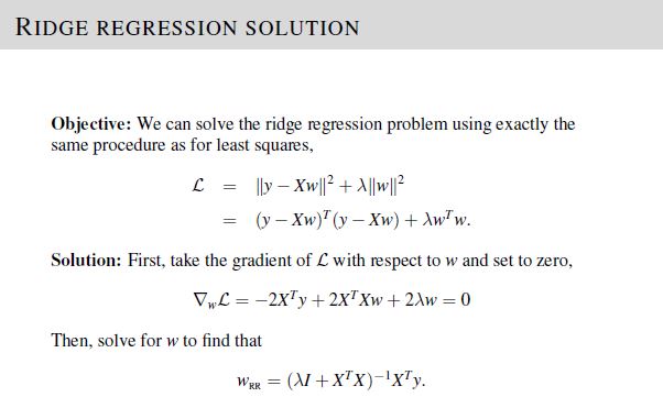
In part 1 of the project, we are required to compute the ridge regression weights \(w_{RR}\) given values of \(y\), \(\mathbf{X}\), and lambda \(\lambda\).

To solve, implement the equations given in Lecture 3, Slide 23.

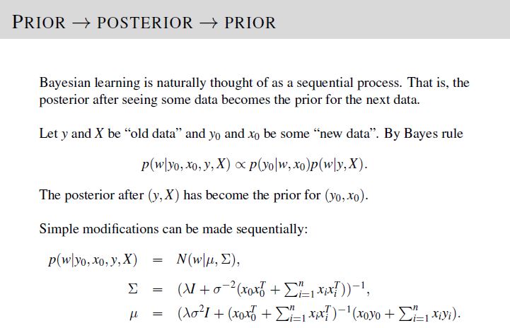
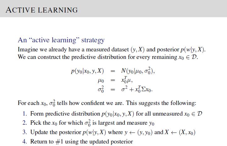
In part 2 of the project, we are required to give 10 data points to measure given values of \(y\), \(\mathbf{X}\), \(\lambda\), and \(\sigma^2\), via active learning procedure.

To solve, implement the active learning procedure given in Lecture 5, Slide 18 and update the posterior distribution following the equations in Lecture 5, Slide 16.

Points to note:

• No preprocessing or normalization of the data is required
• No need to remove the column of 1’s
• Use 1-based indexes for the position of the data point \(\left(y,\mathbf{x}\right)\) to be measured

The test data set and desired output was generated using the following parameters:

\[\begin{align} \text{dimension of vector }\mathbf{x}_i\text{, } d & = 3\\ \text{covariate vectors in }\mathbf{X}_{train}\text{, } n_{train} & = 1000 \\ \text{variance, }\sigma^2 & = 3 \\ \text{lambda, }\lambda & = 2 \\ \text{ true }\mathbf{w} & = \left[2, 3, 4\right]\\ \text{covariate vectors in }\mathbf{X}_{test}\text{, } n_{test} & = 100 \\ \end{align}\]

Week 6 Project: Classification

We are required to implement a \(K\)-class Bayes classifier to compute the probability of a new data point belonging to each of the \(K\)-class. To achieve this, we also need to compute the class prior probability \(\hat{\pi}_y\), class-specific Gaussian mean \(\hat\mu_y\) and covariance \(\hat\Sigma_y\).

To solve, implement the equations given in Lecture 7, Slide 27.

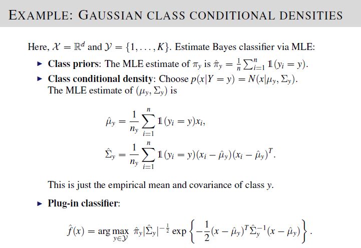
The test data set and desired output was generated using \(K = 6\) classes having index values \(0,1,2,...,5\). A smaller number of classes was used to simplify simulation data. After verification, please reset number of classes \(K = 10\) in your code before submission.

Week 9 Project: Clustering

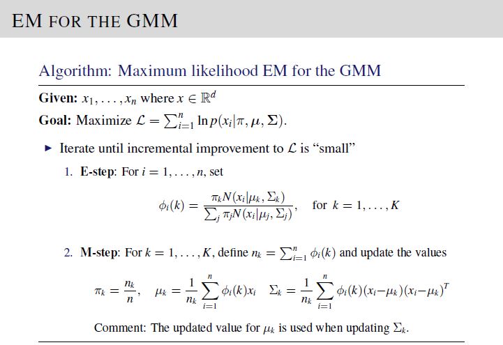
We are required to implement K-means clustering and EM Gaussian Mixture Models on a set of input covariate vectors \(\mathbf{x}_i\). To solve, implement the equations on Lecture 14, Slide 15 and Lecture 16, Slide 20 for K-means clustering and EM GMM, respectively.

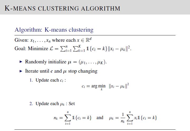
The test data set and desired output was generated using \(K = 3\) , to simplify simulation. After verification, please reset number of clusters to 5 in your code before submission.

For K-means clustering algorithm, in order to match your code output with the provided desired output file, please use the following initialization. Here, \(\text{mu}=\left[\mu_1; \mu_2; \mu_3\right]\).

mu = np.array([[5.72316172633, 7.03506602245], 
               [0.0887880161461, 3.5291769851], 
               [5.5084357544, 10.4242009312]])

For EM GMM algorithm, in order to match your code output with the provided desired output file, please use the following initialization. Here, \(\text{mu}=\left[\mu_1; \mu_2; \mu_3\right]\), \(\text{piClass}=\left[\pi_1,\pi_2,\pi_3\right]\), and \(\text{Sigma[:,:,i]}=\Sigma_i\)

mu = np.array([[-0.0407818979679, 0.350655592545],
               [1.03391556709, 8.99950591741],
               [5.92093526532, 8.10258914395]])
piClass = np.array([0.359950569514, 0.305602403093, 0.334447027393])
Sigma[:,:,0] = np.array([[0.766841596490151, 0.15545615964593],
                         [0.15545615964593, 2.70346004231149]])
Sigma[:,:,1] = np.array([[4.48782867349354,	1.69862708779012],
                         [1.69862708779012,	3.18750711550936]])
Sigma[:,:,2] = np.array([[4.26557534301669,	1.29968325221235],
                         [1.29968325221235,	4.32868108538196]])

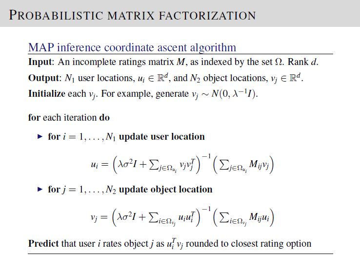
Week 12 Project: Matrix Factorization

We are required to implement the probablistic matrix factorization (PMF) model. To solve, implement the equations on Lecture 17, Slide 19.

The test data set provided has 1200 rows of ratings, with Nu = 100 users and Nv = 100 objects.

For PMF algorithm, in order to match your code output with the provided desired output file, please use the following initialization. Here, \(\text{dim}=d\), \(\text{mu}=\mu\), \(\text{variance}=\sigma^2\), \(\text{lambdaParam}=\lambda\), \(\text{Umatrix}=\mathbf{U}\), and \(\text{Vmatrix}=\mathbf{V}\)

dim = 5 #matrix dimension U = Nu x dim, V = Nv x dim
mu = 0
variance = 1/10
lambdaParam = 2
Umatrix = np.zeros((Nu,dim)) #Initialize Umatrix of size Nu x dim

Additionally, initialize Vmatrix of size Nv x dim by the values provided in the file “Vmatrix_initial_values.csv” in the project repository.

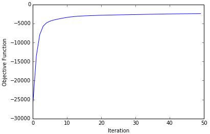
Shown below is the maximization of the log joint likelihood objective function versus iteration number, produced by my Python solution for this project.